Wind Turbine Surface Damage Detection using Deep Learning Algorithm

In this article, I will be detailing out how deep learning algorithm such as Faster-RCNN can be used to detect wind turbine blade damages from the drone images. I used Keras to implements this solution.

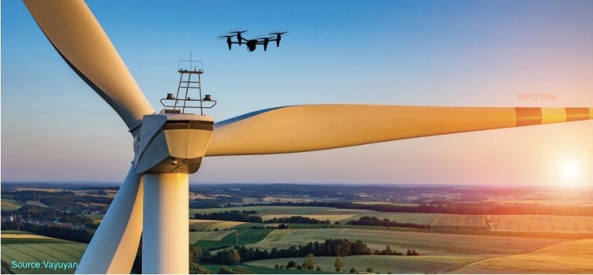
Timely detection of surface damages on wind turbine blades is imperative for minimizing downtime and avoiding possible catastrophic structural failures. A large number of high-resolution images of wind turbines which are taken from a drone, are routinely acquired and subsequently analyzed by experts to identify imminent damages.  Automated analysis of these inspection images with the help of deep learning algorithms can reduce the inspection cost and maintenance cost.

Data

      I used data from a publicly-available drone inspection image of the “Nordtank” turbine over the years of 2017 and 2018. The dataset is hosted within the Mendeley public dataset repository.

Annotation

Using Labelimg, I manually annotate each image, which contains contained at least one wind turbine. Annotating the images in Labelimg creates an XML file corresponding to each image. These XML files must be converted to CSV and then TFRecords. Full code of this step available in my notebook.

To simplify the illustration, I just used the Vortex Panel, Vortex Panel Missing teeth, and Surface Damage as the type of defects to detect by the model. A few of the labeled images are shown below. In total, 320 (182 had positive samples) images were used for training and 63 for testing.

Table: Manual Annotation counts

Defect Type	Training	Testing
Surface Damage	237	40
Vortex Panel Missing teeth	116	40
Vortex Panel	210	70

I randomly split images for training and testing to separate folders and generated annotated files from the annotation xml with bounding box coordinates in a specific format that needed for faster-RCNN model. Annotate file contains the image name with full path, defect type and bounding box coordinates for each image. There can be multiple rows for one image as a single image can have more than one defect type.

Image_name,x1,x2,y1,y2,defect_type

Here are few samples of annotated turbine images

Approach

Faster R-CNN model

Faster R-CNN is an updated version of R-CNN (and Fast R-CNN). The structure is similar to Fast R-CNN, but the proposal part is replaced by a ConvNet.

      Faster R-CNN architecture

Convolution layer converts images into high-level spatial features called the feature map. Region Proposal Network (RPN) on these feature maps and get estimate where the objects could be located and ROI pooling is used to extract relevant features from the feature map for that particular region and based on that classifier, making the decision of whether an object of that particular class is present or not in the fully connected layer.

I adopted the faster RCNN implementation from keras-frcnn. I modified the parameters and image resolutions, prediction results for this problem. In the faster-RCNN model, the base network is ResNet. And the RPN built on the base layers. In addition, we have the classifier also built on the base layers

# base layers
shared_layers = nn.nn_base(img_input, trainable=True)
# define the RPN, built on the base layers
rpn = nn.rpn(shared_layers, num_anchors)
# define the classifer, built on the base layers
classifier = nn.classifier(shared_layers, roi_input, C.num_rois,
 nb_classes=len(classes_count), trainable=True)
# defining the models + a model that holds both other models
model_rpn = Model(img_input, rpn[:2])
model_classifier = Model([img_input, roi_input], classifier)
model_all = Model([img_input, roi_input], rpn[:2] + classifier)

Mean Average Precision

I used the Mean Average Precision (MAP) to measure the quality of prediction. MAP is commonly used in computer vision to evaluate object detection performance during inference. An object proposal is considered accurate only if it overlaps with the ground truth with more than a certain threshold. Intersection over Union (IoU) is used to measure the overlap of a prediction and the ground truth where ground truth refers to the original damages identified and annotated.

The IoU value corresponds to the ratio of the common area over the sum of the proposed detection and ground truth areas (as shown in above image)

Training

 I have used 182 annotated images that were used for training and 63 for testing. For all image and model preprocessing, I used my Jupyter notebook (available in my GitHub) and for training and testing the faster-RCNN model in GPU, I used google Colab environment.

./train_files/DJI_0052.JPG,1538,2541,1656,2668,SURFACE_DAMAGE_TY1

./train_files/DJI_0126.JPG,3555,2487,3574,2497,SURFACE_DAMAGE_TY1

./train_files/DJI_0127.JPG,4693,368,4737,408,VG_MISSING_TEETH

After making the annotation file in the above format, process  training using below script

python train_frcnn.py -o simple -p train_annotate10.txt

It might take a lot of time to train the model and get the weights, depending on the configuration of your machine. I suggest using the weights I’ve got after training the model for around 60 epochs. You can download these weights from my GITHUB.

Here is the plot of my training accuracy and losses during training each epoch.

Prediction

Now the training is completed and I do see the optimal accuracy and loss coverage around 25 epoch. The classification accuracy is 98% and it a great score. Let us start to predict with unannotated images. After move the testing images to test_files call the test_frcnn.py script below

python test_frcnn.py -p test_files

Finally, the images with the detected objects will be saved in the “results_imgs” folder. Below are a few (full data available in my GitHub) examples of the predictions I got after implementing Faster R-CNN:

The model predicted VG Panels, Missing Teeth, and Surface Damage in the validation image set are detected with high probability with the default training parameters as you see in the resulted images. However, I’ve found that many actual VG panels not detected when it was a different angle, or not correct zoom level.  I am sure adding more samples will solve this and improve the model’s efficiency.

Conclusion

Faster RCNN model did great with respect to my sample data. Mean Average Precision (MAP) is good for the model when it predicted the defect surface. However, the model did not get to detect all missing panel teeth scenarios. Also, I have not considered this model, due to a lack of training images for this particular type. This faster-RCNN deep learning model will greatly improve efficiency when we add many training samples and images taken from different climatic conditions. In addition, we need custom augmentation methods to make a lot more training samples than standard augmentation techniques.

I will update my progress with another article soon. You can access the Jupyter notebook with full code for detecting wind turbine surface defects in my GitHub

References:

1.     This is the research paper inspired me for this article: Wind Turbine Surface Damage Detection by Deep Learning Aided Drone Inspection Analysis

2.     Data Source: DTU - Drone inspection images of wind turbine